Transformer (Self Attention)
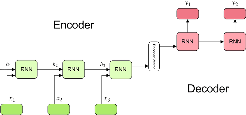
Whenever long-term dependencies (natural language processing problems) are involved, we know that RNNs (even with hacks like bidirectional, multi-layer, memory-based gates — LSTMs/GRUs) suffer from vanishing gradient problem. Also, they handle the sequence of inputs 1 by 1 or word by word this resulting in an obstacle towards parallelization of the process. Especially when it comes to seq2seq models, is one hidden state enough to capture global information about the translation? To solve this type of issue we use the Attention mechanism along with the seq2seq model. The below figure represents the conventional encoder-decoder model architecture.
Now let’s try to interpret the Attention mechanism.
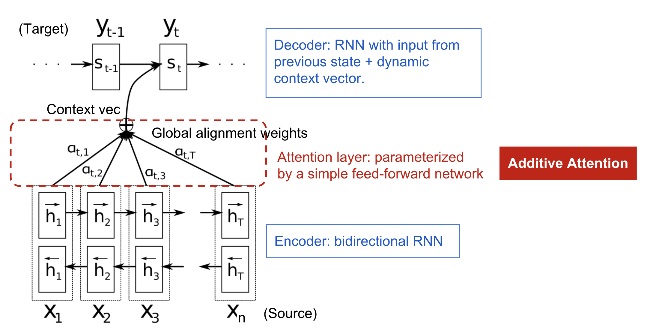
Encoder-Decoder With Attention Mechanism Layer Bahdanau et al., 2015.
The main idea here is to learn a context vector \(c_i\), which gives us global level information on all the inputs and tells us about the most important information. For eg. In the case of the machine translation task, let’s say if we are translating from french to the English language then this context vector tells us which words from the input text to pay attention to or tells us the importance of each word from the context window while generating the current English output word. Following is the mathematical representation of the attention layer.
The context vector \(c_i\) is computed as a weighted sum of all the inputs.
$$c_i = \sum_{j=1}^{Tx} \alpha_{ij} h_j$$
The weight of \(\alpha_{ij}\) is computed using:
$$\alpha_{i_j} = \frac{exp(e_{ij})}{\sum_{k=1}^{Tx} exp(e_{ik})}$$
S.T.
$$\alpha_{ij} >= 0, \alpha_{ij} = \sum_{j=1}^{Tx} \alpha_{ij} = 1$$
Where,
$$e_{ij} = a(s_{i-1}, h_j)$$
function \(a\) is a simple 1 layer feed-forward neural network.
The attention mechanism solves the problem of the long term dependencies by allowing the decoder to “look-back” at the encoder’s hidden states based on its current state. This allows the decoder to extract only relevant information about the input tokens at each decoding, thus learning more complicated dependencies between the input and the output.
The following graph is the BLUE score comparison between the attention model vs the conventional encoder-decoder model. As we can observe, with the attention layer even after the word limit exceeded above 30 or 50 words performance of the model did not drop compared to the rest of the model.
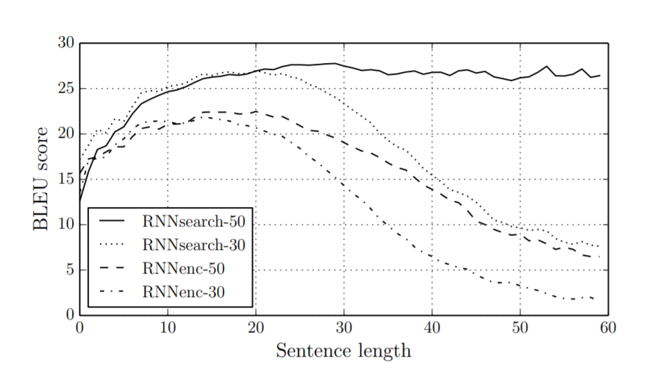
BLEU Score Comparison
RNNseach: Encoder-decoder model with attention layer.
 RNNenc: Encoder-Decoder model without attention layer.
But, Why do we need the Transformer?
RNN based encoder-decoder models work quite well for the shorter length sequences and to handle long term dependencies we can add the attention layer. But these models are very hard to parallelize. Because to generate the output sequence first we need to generate the context vectors which are generated from the input sequence and these inputs sequences are fed to the encoder part of the model one by one not all at once. In a way, the RNN based model creates heavy dependencies on the previous inputs because of which it becomes very hard to process them parallelly.
In the Transformer architecture of the encoder part, all the input sequences are fed all at once instead of ingesting them one by one. We’ll discuss this in more detail later.
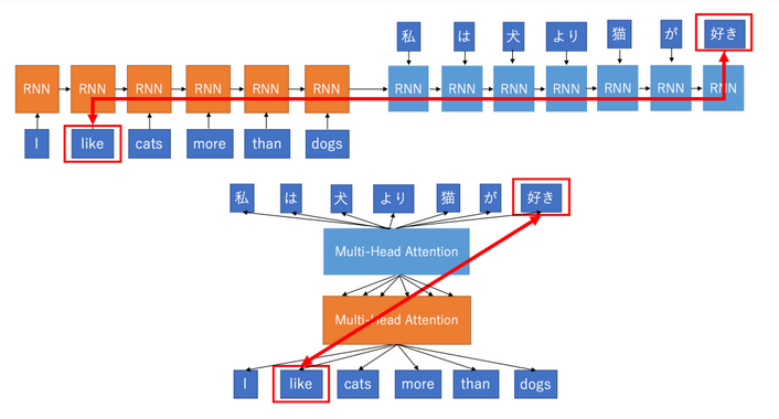
To solve this problem of RNN based model people also tried CNN based models, which are very trivial to parallelize and they also fit the intuition that most dependencies are local. The reason why Convolutional Neural Networks can work in parallel is that each word on the input can be processed at the same time and does not necessarily depend on the previous words to be translated. Not only that, but the “distance” between the output word and any input for a CNN is in the order of log(N) — that is the size of the height of the tree generated from the output to the input (ref below figure). Which is much better than the distance of the output of an RNN and input, which is on the order of N.
But the Convolutional Neural Networks does not necessarily help with the problem of figuring out the dependencies when translating sentences. That’s why Transformers were created, as they are a combination of CNNs with attention.
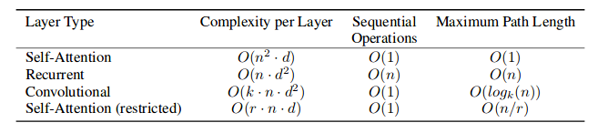
Time complexity
Advantages of Transformers over CNN and RNN model
- Parallelization of Seq2Seq: RNN/CNN handle sequences word-by-word sequentially which is an obstacle to parallelize. Transformer achieves parallelization by replacing recurrence with attention and encoding the symbol position in the sequence. This, in turn, leads to significantly shorter training time.
- Reduce sequential computation: Constant O(1) number of operations to learn dependency between two symbols independently of their position distance in sequence.
Encoder and Decoder Stacks in Attention is all you need (As per the paper)
Encoder
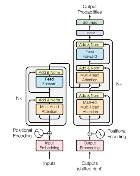
The encoder is composed of a stack of N=6 identical layers. Each layer has two sub-layers. The first is a multi-head self- attention mechanism, and the second is a simple, position-wise fully connected feed-forward network. We employ a residual connection around each of the two sub-layers, followed by layer normalization. That is, the output of each sub-layer is LayerNorm(x+ Sub layer(x)), where Sub layer(x)is the function implemented by the sub-layer itself. To facilitate these residual connections, all sub-layers in the model, as well as the embedding layers, produce outputs of dimension = 512.
Decoder
The decoder is also composed of a stack of N= 6 identical layers. In addition to the two sub-layers in each encoder layer, the decoder inserts a third sub-layer, which performs multi-head attention over the output of the encoder stack. Similar to the encoder, we employ residual connections around each of the sub-layers, followed by layer normalization. We also modify the self-attention sub-layer in the decoder stack to prevent positions from attending to subsequent positions. This masking, combined with the fact that the output embeddings are offset by one position, ensures that the predictions for position i can depend only on the known outputs at positions less than i.
In General we can think of Encode-Decoder architecture as
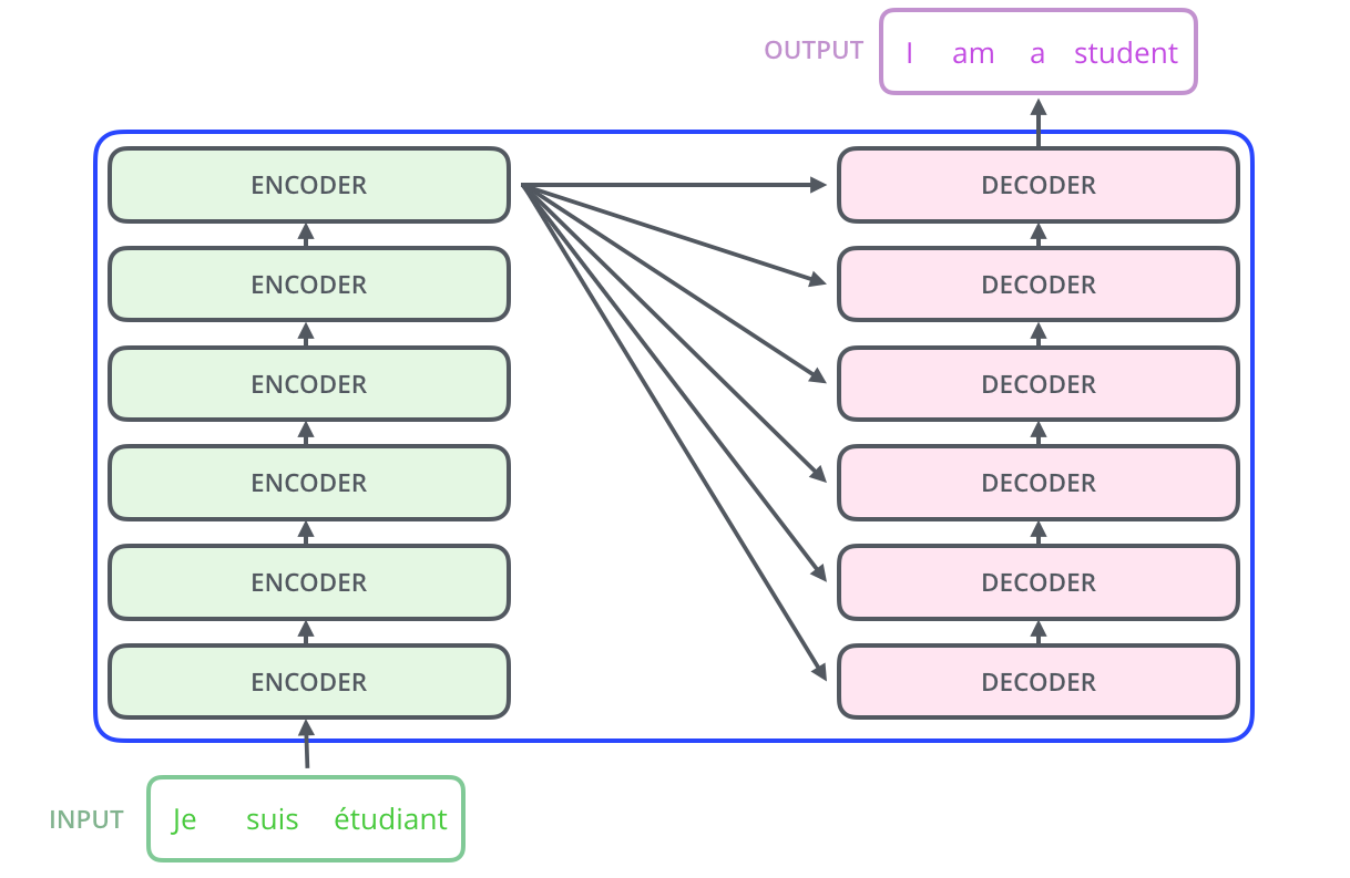
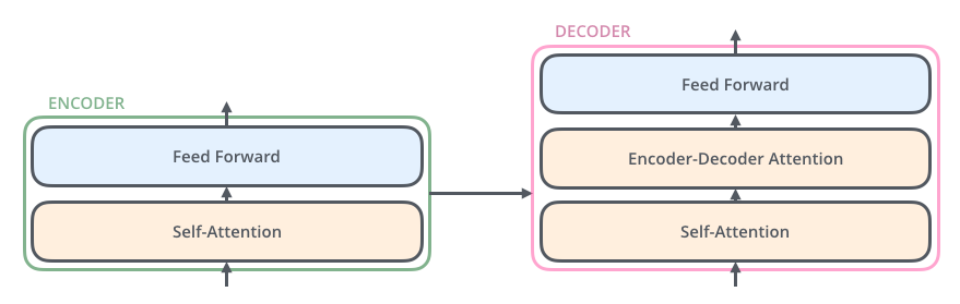
In general, all the encoders are very similar with the same architecture in which there are two layers: Self-attention and a Feed Forward Neural Network. Individual encoder-decoder architecture is shown below:
- The encoder’s inputs first flow through a self-attention layer. It helps the encoder look at other words in the input sentence as it encodes a specific word.
- The decoder includes self-attention and feed-forward neural network with an attention layer between them that helps the decoder to focus on relevant parts of the input sentence.
Self Attention (As per the paper)
An attention function can be described as mapping a query and a set of key-value pairs to an output, where the query, keys, values, and output are all vectors. The output is computed as a weighted sum of the values, where the weight assigned to each value is computed by a compatibility function of the query with the corresponding key.
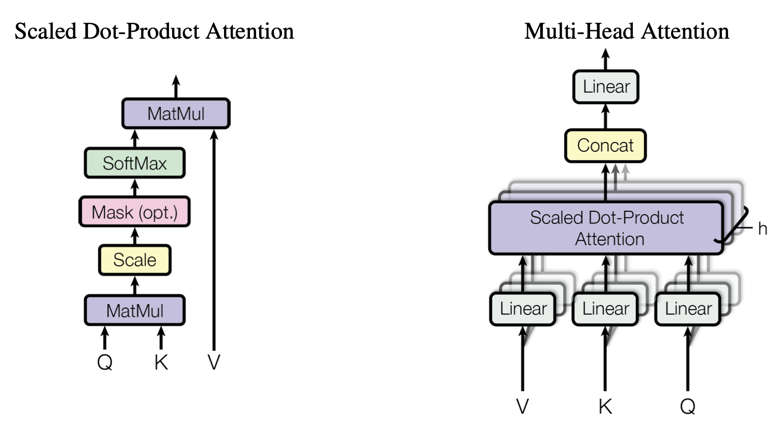
Instead of performing a single attention function with \(d_{model}\)-dimensional keys, values, and queries, we found it beneficial to linearly project the queries, keys, and values \(h\) times with different learned linear projections to \(d_k\), \(d_k\) and \(d_v\) dimensions, respectively. On each qkv of these projected versions of queries, keys, and values we then perform the attention function in parallel, yielding d dimensional output v values. These are concatenated and once again projected, resulting in the final values, multi-head attention allows the model to jointly attend to information from different represent at ion subspaces at different positions. With a single attention head, averaging inhibits this, as depicted in below Figure:
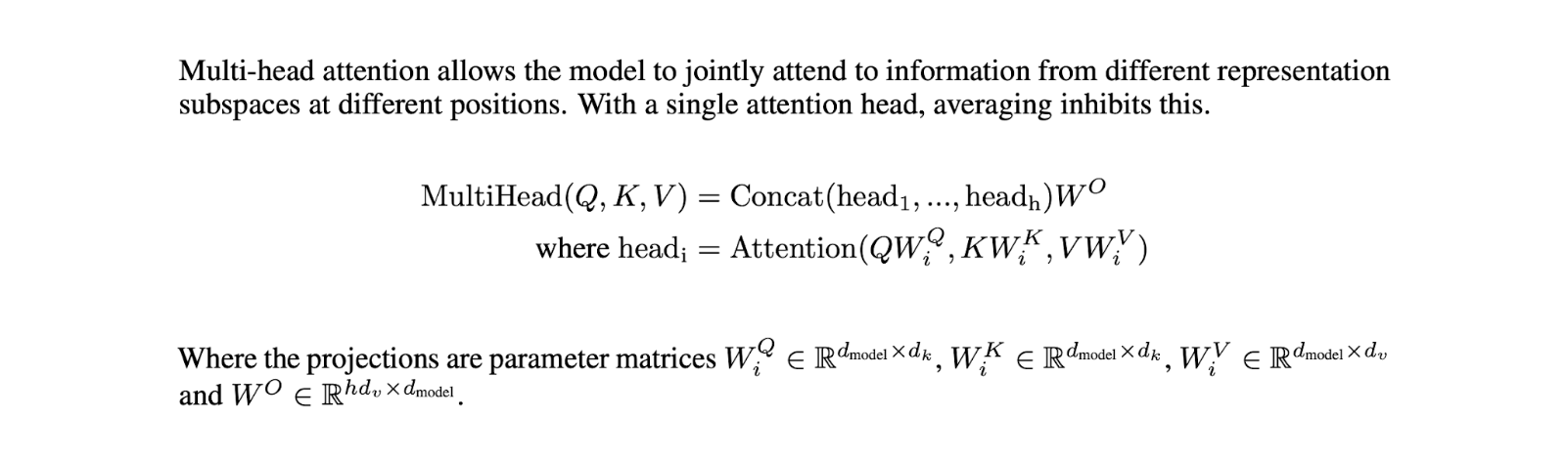
In this work, \(h= 8\) parallel attention layers, or heads. For each of these we use \(d_k = d_v =d_{model} / h = 64\) . Due to the reduced dimension of each head, the total computational cost is similar to that of single-head attention with full dimensionality.
Demystifying self-attention
- The input to the self-attention layer is nothing but the word embeddings of 512 dimensions. This embedding happens for only the bottom-most encoder because the self-attention layer creates its representation of the word embeddings as shown below:
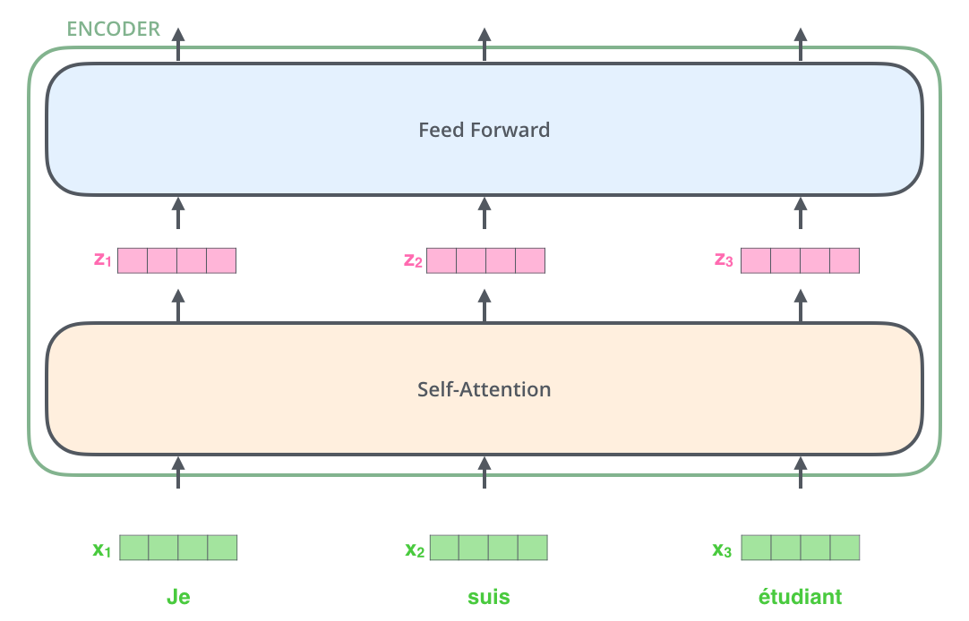
- For the first encoder input will be word embeddings and output is fed as input to the next encoder.
- In the above encoder architecture as you can see each input is flowing through its path, but they have their dependencies in the self-attention layer. Whereas the feed-forward network part has no such dependencies, because of which several paths can be executed in parallel while going through the feed-forward network.
Following calculation steps are followed in the self-attention layer:
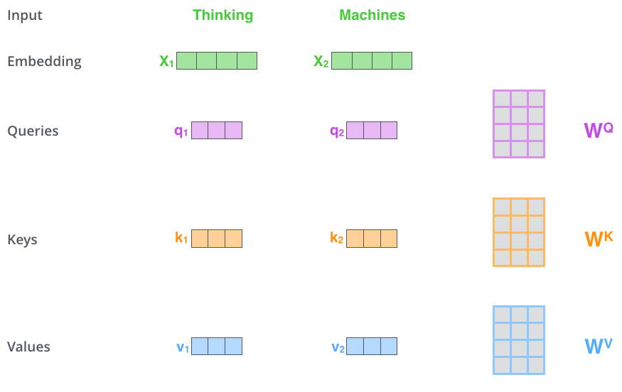
- We create vectors query(q), key(k) and value(v) by multiplying input vectors with matrices Wq, Wk and Wv respectively and these matrices are updated during the training process and these vectors are of smaller dimension (dim=64) as compared to input embeddings dimension (dim=512).
- From the computed query (q) and key (k) vectors, we compute a score by performing dot product between two vectors. This score represents the importance of each word w.r.t. The targeted word (word1=” Thinking”). We do this task for every input token as shown in the below figure.
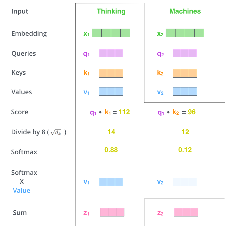
- In the next step we divide the scores by 8 (square root of the dim=64, it’s the default score as per the paper), then we pass the normalized score to softmax to generate output between 0 to 1. So that we can represent the percentage of attention that each token contributes w.r.t. to the targeted word. As we can see in the above figure. the targeted words softmax score will be very high as compared to the rest of the words.
- Now we multiply each value vector (v) by the softmax score and we add all the values vectors to generate vector z. The idea here is to keep the value of the targeted word and the words we want to focus on, by performing a summation of the value(v) vectors. In this, the irrelevant words vector will have little impact on the z score calculation and the more relevant words and the current word will have a much greater impact on the Z score at the end.
Decoder
- From the top encoder’s output we get the representations of each of the tokens and the output representations are used to generate \(K_{encdec}\) and \(V_{encdec}\) . These matrices are computed by multiplying them with Wk and Wv respectively. The attention vector \(K_{encdec}\) and \(V_{encdec}\) is fed to each decoder block’s “encoder-decoder attention” layer to pay attention to the input sequence while generating the current output token. Now, let’s try to understand the decoder stack architecture.
- Architecture of decoder block is quite similar to an encoder with one Masked self-attention layer and the feed-forward network layer. Apart from these two layers it also has one more encoder-decoder attention layer in between them. Lets now understand each layer one by one.
- Similar to the encoder’s input, we embed and add positional encoding to the decoder inputs.
- In the First masked self-attention layer, the decoder pays attention to the only previous position in the output sequence, because we generate the output sequence one by one in the decoder stack. So we have only previous output tokens to focus on and we also mask the future output positions by -inf.
- In the encoder-decoder attention layer, We take query vector Q from the previous layer and use vectors \(K_{encdec}\) and \(V_{encdec}\) generated from the output of the top encoder to complete the whole attention mechanism computation and to generate each tokens representation.
- Now, the generated representations are fed to the feed-forward network. So the output of the last decoder block is ingested into a linear softmax layer which generates the output and the output is again used as one of the inputs to the decoder to generate the next token words and the process repeats until the special token symbol does not appear.
Multi-Head Attention
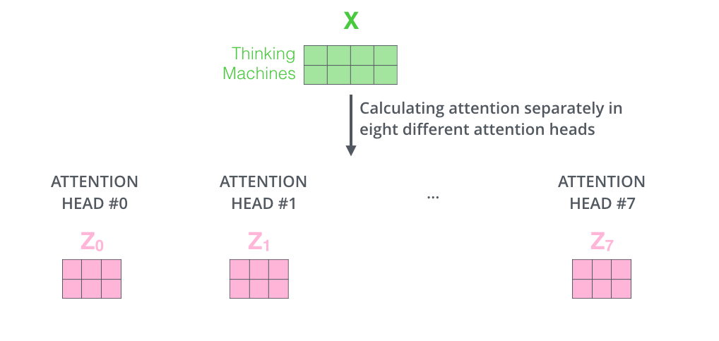
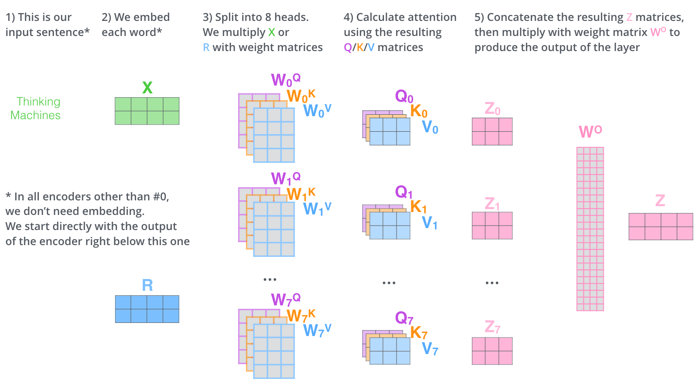
Multi-head attention is nothing but performing the self-attention calculation multiple times (eight times) with just different weight matrices Wq, Wk & Wv. With this, we will end up with multiple Z values (eight).
Now that we’ve eight different vectors for Z, but as we have seen in the architecture that we get one representation per tokens as the end output of the encoder. So to get a single vector as the output \(z\), we concatenate all the eight different \(z\) vectors and then we multiply it by a weight matrix \(W_0\) Which also gets updated during the model training process.
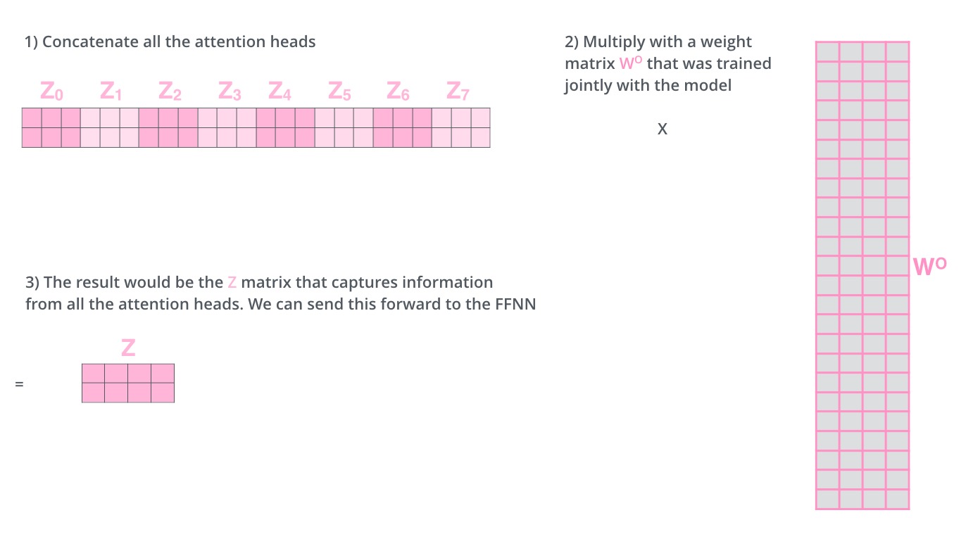
The below figure shows the entire process of the multi-head attention layer.
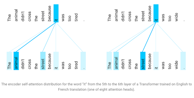
As we have seen that the Multi-Head Attention is just several attention layers stacked in parallel, with different linear transformations of the same input. So that model can visualize other parts of a sentence when processing or translating a given word, it gains insights into how information travels through the network. Visualizing what words the encoder attended to when computing the final representation for the word “it” sheds some light on how the network made the decision. In its 5th step, the Transformer relates the word “it” with two nouns “animal” and “street”. Both words could relate to the word “it” in a different context. But the word “it” relates to “animal” more than “street” in the left sentence figure, but in the right sentence “it” clearly relates with the word “street” more. The transformer learns all these differences in the next layer.
Conclusion and Further Readings
This blog demonstrates that self-attention is a powerful and efficient way to replace RNN as a method of modeling dependencies. I highly recommend you to read the actual paper for further details on the hyperparameters and training settings that were necessary to achieve state-of-the-art results and also you can read Jay Alammar blog on The Illustrated Transformer.